In the Worst-case Tolerance Stack-up Analysis article, you will read about worst-case or linear stack-up analysis. Such an analysis assumes that all dimensions in the tolerance chain have worst-case deviations from their nominal values. A statistical tolerance stack-up analysis considers the probability of a tolerance value and the combination of tolerances. It turns out that the probability of a worst-case combination is negligible for even a small number of parts. Let’s look at the following example.
Suppose you are making a stack of 4 identical parts and you want to analyze the total height of the stack. The parts have a height specification of 10 +/-1. Now assume that all parts have a worst-case deviation and are either 9 (part ‘9’) or 11 (part ’11’) high (any dimension, mm, inch, meter, etc.). With only 4 parts, it is still possible to write down all possible combinations.
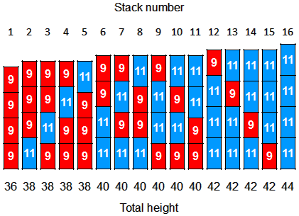
So, there are 16 possible combinations.
The probability of an extreme thickness is 2/16 = 12.5%. If, for example, only the top pile is problematic, the probability is only 6.25%. Note that this is an extreme tolerance distribution with a low probability itself. In practice, the probability of an extreme height is very low.
It is clear that it is beneficial to consider the probability distribution of the tolerances and perform a statistical analysis
.
Distribution of Tolerances
In the worst case example above, there was an extreme distribution of tolerances. The question now is what is a (more) realistic distribution. This is not an easy question to answer, but a better estimate would increase the accuracy of your analysis.
If similar parts have been produced, you have important data to make a good estimate of the tolerance distribution. But what if you’re working on a new product and don’t have that kind of data to compare?
Normal Distribution of Tolerances
If you don’t know the distribution of tolerances, you have to make an estimate. It is often assumed that tolerances have a normal (Gaussian) distribution. This is because the normal distribution seems to occur in “almost all cases”. In statistics, this is called the central limit theorem. Roughly speaking, this theorem states that “the sum of a large number of independent and identically distributed random variables, will be approximately normally distributed“. Since the manufacturing process of machined parts consists of many variables, it is safe to assume a normal distribution of tolerances. An added benefit is that it is relatively easy to add up normally distributed tolerances.
A common assumption is that the tolerance limits coincide with the +/-3σ (3x standard deviation) values. As a reminder, the standard deviation is a measure of variation. 99.7% of the population falls within the +/-3σ limits.
.
Statistical Stack-up Tolerance Analysis
A widely used method for performing a statistical stack-up tolerance analysis is the Root-Sum-Squares (RSS) method. Variances (the standard deviation is the square root of variance) can be added. This makes it easy to sum normally distributed tolerances: Ttot = √(T12 + T22 + …. Tn2).
In the example above, all tolerances were +/-1, so the total height variation is: Ttot = √(12 + 12 + 12 + 12) = 2. The stack of parts will have a height of 40 +/-2. And 0.3% of the stacks will be smaller or larger (with a height of 36 .. 38 or 42 .. 44).
Tolerance Analysis Stack-up Spreadsheet
A tolerance analysis spreadsheet is available in the Engineering Toolkit of Vink System Design & Analysis. This allows you to quickly start performing tolerance analysis, including the statistical method described here. The advanced method as described in ‘Advanced Method of Tolerance Analysis‘ is also possible.
In a next article I will discuss how realistic a normal (Gaussian) distribution is.