The article ‘Setting up the tolerance chain step-by-step‘, described how to set up a tolerance chain step-by-step using an example. The article ended with a sketch of the tolerance chain. You can see this chain in the figure below. By processing the part dimensions with tolerances using (for example) TolStackUp, you get a complete tolerance analysis.
Working Out a Tolerance Chain with Dimensions and Tolerances
Let’s work out this example with numbers and enter them into the TolStackUp spreadsheet. This completes the tolerance analysis. I assume the following (arbitrary) values:
- P = 4 +/-0.1
- R = 8 +0.2/0
- B = 21 +/-0.1
- H = 10 +0.1/-0.15
When you enter these data and names in the tolerance pool (columns H, I, J), it looks like in the figure below. Note that the ‘House’ tolerance is shown rounded off, but the actual value of +/-0.125 mm will be used in the calculations.
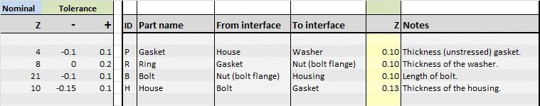
Tolerance Pool Table.
Fill in the Tolerances in the Table
All you have to do now is enter the 4 codes (P, R, B, H) in column B of the tolerance table (Tolerance Chain sheet). The tolerance pool data and the total sum appear immediately. For clarity, I have removed some (mostly empty) rows and columns:
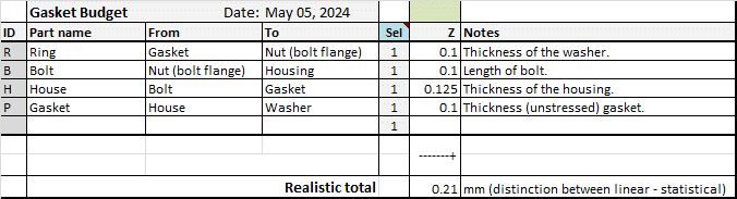
Tolerance table result.
To evaluate whether the selected tolerances are satisfactory, you must create and fill in the specifications. To complete the example, I suggest the following specifications:
- The minimum compression for a good seal is 0.8 mm;
- To avoid damaging the gasket, the maximum compression is 1.3 mm.
How Do You Fill in the Specification?
To fill in the specification, first look at the nominal compression. You can see this nominal compression by expanding columns F through Q in the spreadsheet. Below you can see a small section. Also note how you (manually) specify the ‘direction’ of the absolute dimension in column J.

Calculation nominal dimension.
You can see that the nominal compression is 1.075 mm. You might have expected exactly 1 mm, but because of the asymmetric tolerance of the Ring and the House, the expected compression is slightly higher. So, based on this analysis, the compression of the gasket is 1.075 +/- 0.21 mm.
Now we can determine the specification and enter it into the spreadsheet:
- Minimum compression requirement: 0.8 mm – 1.075 mm = -0.275 mm.
- Requirement for maximum compression: 1.3 mm – 1.075 mm = 0.225 mm.
Enter these two specifications and you’ll see the overall result.
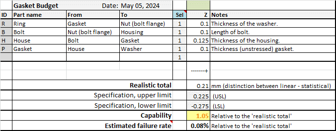
Result and capability.
What Conclusions Can Be Drawn?
The following conclusions can be drawn:
- The four tolerances combined are just sufficient. The capability (1.05) indicates that there is only a 5% margin over specification.
- The estimated failure rate is 0.08%.
- The lower and upper specification limits are not equal. This means that the nominal dimension(s) of the parts are not optimal.
Note that the above analysis and conclusions are based on the assumption that the tolerances are Normally distributed and that the 3σ values are exactly equal to the tolerance requirements on the drawing. This assumption will never be completely correct in practice.
What Improvements Can Be Made?
There is (too) little margin between the expected variation and the specification. Especially since it is not clear that the above assumption is correct. One improvement is fairly easy to implement: adjust the nominal compression of the gasket to be exactly halfway between the two specification limits. The nominal compression should then be: (0.8 mm + 1.3 mm)/2 = 1.05 mm.
It does not matter which part you adjust. I will use the ‘House’ as an example, which then gets a thickness of 9.975 -0.15/+0.1 mm. analysis shows that the capability increases to 1.17 and the failure rate is halved.
The second improvement might be to reduce one or more of the tolerances. Again, this is fairly easy to do. But another possibility is to produce the parts using a controlled process, an SPC process. Such an SPC process is particularly suitable for mass production. Let’s see what it can do for this example.
SPC Tolerance Analysis
SPC tolerance analysis differs from standard analysis in that SPC tolerance analysis assumes that the parts in the construction are produced with ‘SPC requirements’. Therefore, an SPC tolerance analysis is not very different from a standard analysis. All you have to do is enter the exact same numbers in TolStackUp’s ‘SPC-TolerancePool’ sheet. And enter the codes in the/a table in the ‘SPC Tolerance Chain’ sheet.
Below are the results, first the SPC tolerance pool and then the corresponding tolerance table. The only adjustment made is the nominal dimension of the ‘House’. This was changed from 10 mm to the 9.975 mm suggested above. The standard set requirements of Cpk = 1.5 and the maximum allowable deviation from the mean μ = 1.5σ are the default in TolStackUp, but you can use any value in the spreadsheet. These defaults are the same as the 6 sigma requirements.
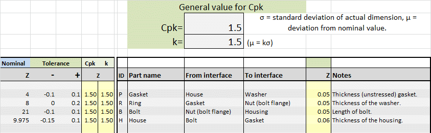
SPC tolerance pool.
And this is the complete SPC tolerance analysis:

Now you see three things:
- The lower and upper limit specifications are the same (absolute value). So the nominal dimension is just right within the specified requirements.
- The Cpk = 1.47 and the color is red. The red color is because the TolStackUp spreadsheet automatically sets the same requirement for the outcome as the requirement for the constituent parts. Of course, you can change this to suit your needs.
- The estimated failure rate has dropped from 0.08% to 0.0005%, 16 times lower.
This result is much better (lower failure rate) but also more reliable. The higher reliability of the analysis result is due to the Cpk requirements on the components.
Conclusion
Once you have set up a tolerance chain, a tolerance analysis with TolStackUp is quick and easy to do. The result of the analysis gives you immediate insight into the design and what can be improved. The application of SPC, results in a much higher reliability of both production and your tolerance analysis.