A previous article described the entire step-by-step plan for building a tolerance chain. It was described using a relatively simple example. In practice, however, designs can be much more complex. And then the tolerance analysis of such a design is much more complicated. But even for a relatively simple design, tolerance analysis can be difficult. Therefore, here is a simple clamping mechanism to further illustrate a more complicated tolerance analysis process.
When creating a tolerance chain, you may encounter structural elements that are difficult to include at first glance. Common elements include springs, levers, and clearance. Here is an example that includes two of these elements.
A Simple design, but a Difficult Tolerance Analysis
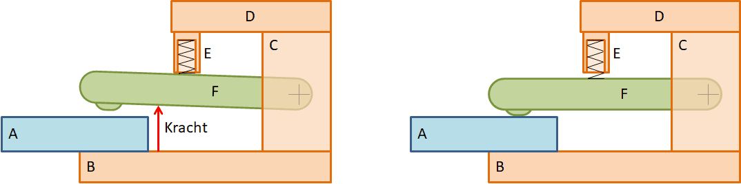
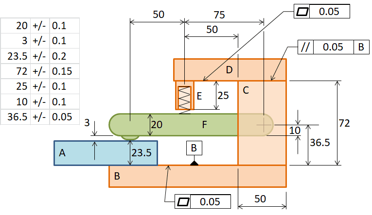
The design is a mechanism for clamping plates in an automated manufacturing process. The clamping force is applied by a spring. When the manufacturing step is complete, a counterforce causes the clamp to open. The plate “leaves” the clamp and a new plate slides into the clamp. The following two figures show a simple sketch of the design. There is a spring (in part E), a lever (part F) and a clearance. The clearance is not visible in the figure, but is in the pivot of the lever F in column C. Between opening and closing the clamp, the entire clearance is passed through.
Note that this sketch is actually step 3 in the step plan described in Setting up the tolerance chain step-by-step.
Lever-operated clamping mechanism open and closed.
What Can Go Wrong, the Critical Dimension
The question here is not whether this is the most optimal design. There could be any number of reasons for arriving at this design. The question now is to make the tolerance analysis for this design. The first step, step 1, is to determine the critical dimension. To determine this critical dimension, it is usually helpful to ask the question: what can go wrong?
As you can see in the two figures, the clamp can only open a little. One problem that could occur is that plate A does not fit into the clamp when it is open. This is then due to a combination of a “too thick” plate A and other unfavorable tolerances. So the critical dimension will have to do with the opening of the clamp. But let’s look at the machine states before we determine the critical dimension.
Machine States
Step 2 of the step plan deals with machine states. In this clamping mechanism design, there are two states: open and closed. It will be obvious that the closed state is irrelevant to the problem outlined. When the clamp is closed, a plate is already in the clamp and there is no problem. So the problem is the open state.
What Critical Dimension to Choose?
It seems obvious to draw the critical dimension in the sketch in the open state. This is the most logical because it shows the condition in which the problem of a plate not fitting can occur. However, it is also possible to define the critical dimension in the closed condition. The figures below show both. In practice, it does not matter which one you choose. In the tolerance chain, the tolerances are exactly the same. And so the end results (capability and failure rate) are exactly the same.
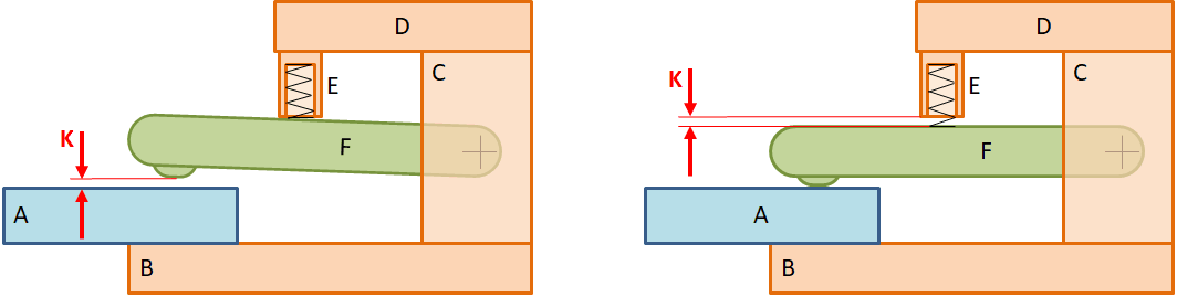
Critical dimension K for open state and for closed state.
Which one you choose is not that important for the final result. But to explain your tolerance analysis to someone else, for example in a review, it is convenient to explain the one for the open state. But sometimes it is easier (for you) to work out the tolerance chain for the other state. Here we choose the critical dimension K in the open state.
The tolerance chain
We have now reached step 4 of the step plan. What the tolerance chain looks like is one of the difficult parts of the analysis. The key is to include all influences on the critical dimension in the chain. An important step is to determine the interfaces of the parts that are part of the chain. Each part in the chain always has two interfaces. And the tolerance chain passes through those two interfaces. But how do you know which interfaces you need in advance if you don’t know the chain yet?
Strategies
If the chain is not immediately obvious, you can use several strategies to determine the tolerance chain:
- Start on one side of the critical dimension and find a way through the structure to the other side of the critical dimension. If you get stuck, continue on the other side of the critical dimension and see if you can reach the point where you left off from that side.
- If you get stuck again, you can try one or more ‘thought experiments‘. Take a part of the structure in your mind and vary a dimension that you suspect is in the chain. Now see if this affects the critical dimension. If so, include that part with that dimension in the tolerance chain. For example, the height of block C. If you increase or decrease the height in your mind, you will see that it affects the critical dimension. So it must be part of the tolerance chain. The tolerance chain must go through this part. Of course, if the design is very complex, you can also do this in your CAD drawing.
- If the design is very complex, you can make a very simplified sketch. In this sketch, you group parts together and represent a group by just one line. This gives you a global tolerance chain. And once you have that global chain, a chain that is closed, then you start to work out the details of the grouped lines.
Doing this for the clamping mechanism results in the tolerance chain shown in the figure below.
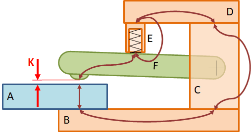
The first part of the tolerance chain.
In short, the elements that contribute are: the height/thickness dimensions of parts A, C, E, and F + the flatness/straightness of parts B and D + the clearance.
But we’re not done yet. The position of the lever pivot also affects the critical dimension. Funnily enough, you now have two paths through the structure, see the figure below. The two paths are marked with a 1 and the added piece with a 2.
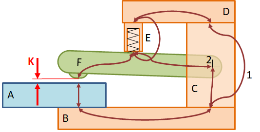
Is this really possible? Yes, creating the tolerance chain is not the final goal, but is useful for collecting all the influences on the critical dimension. The tolerance chain sketch is just a means to get a good tolerance analysis with all contributors.
Interfaces, Dimensions, and Tolerances
Now that you know the tolerance chain, you can use it to collect all the dimensions and tolerances that affect the critical dimension. This is usually not too difficult. If the design already exists, you can look it up. And if the design exists only as a concept, you can determine the dimensions and tolerances yourself. The latter situation is ideal and as it should be: you can choose the best fitting tolerances from the tolerance table! In the figure below, you can see all the dimensions and tolerances involved. In this example, I have chosen symmetrical tolerances, but you can also include asymmetrical tolerances in the TolStackUp template. These asymmetric tolerances will be automatically processed correctly.
The clearance is not shown in the figure, but is given as +/-0.01 mm. As you can see in the sketch above, there are only two arrows in the lever part, one from the pivot point and one to the pressure point for the production plate. The latter, according to the dimensional sketch below, actually consists of two dimensions and tolerances (20 mm and 3 mm). For the sake of clarity, the two are combined into one arrow. But in the tolerance table, they are two contributions!
Dimensions and tolerances of the clamp mechanism.
Filling the Tolerance Table
You can easily enter most dimensions and tolerances into the tolerance table. The TolStackUp tolerance table is excellent for this. The difficulty with this step, however, is how exactly to translate all relevant tolerances into values for the tolerance table. Besides the effect of the lever, we are also concerned with the effect of the flatness of parts B and D, and the effect of the parallelism of part C (0.05 w.r.t. B).
Let’s look at the height dimension (20 mm) of part E, which has a tolerance of +/-0.1 mm. This tolerance acts through the lever (part F), which is amplified in the critical dimension K. This amplification factor is: (50 mm + 75 mm)/(75 mm) = 1.67 (1 2/3). Thus, the contribution of the tolerance of part E is +/-0.1 mm x 1.67 = +/-0.167 mm.
All contributions are explained below in a similar way. We start at the critical dimension K, part A, and then go along the entire chain. You will see that many tolerances are affected by the lever!
The basic idea in determining a single contribution is to vary only that one tolerance (in mind) while ‘holding’ all other dimensions at their nominal values. In other words, in the mind (or CAD), everything is made perfect (to the micron). And only the dimension whose tolerance contribution you want to determine varies in dimension. Then see what happens to the critical dimension.
The individual contributions
- Part A has a single, simple contribution. Nominal dimension 23.5mm with a tolerance of +/-0.1mm.
- Base plate B adds a flatness tolerance. The figure below shows two possible worst cases.
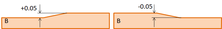
The flatness is specified as 0.05 mm, which translates to +/-0.05 mm in the tolerance table. This variation creates a height variation of the stop point at spring holder E, but the lever pivot also moves with it. Thus, the flatness tolerance has a one-to-one effect on the critical dimension K. - Column C adds three tolerances: height dimension 72 +/- 0.15 mm, parallelism 0.05 mm, and pivot position 36.5 +/- 0.05 mm. Because of the lever, the effect on the critical dimension is different for each tolerance:
– Height dimension 72 +/- 0.15 mm. As a result of this variation in height, there is a variation of +/- 0.15 mm in the height of the stop point at spring holder E. Due to the lever, the effect on the critical dimension is +/- 0.15 mm x (50+75)/75 = +/-0.25 mm;
– Parallelism 0.05 mm. This results in a height variation of the stop point at the spring holder E. The lever follows the stop point at E and the opening for the production plate A (the critical dimension) becomes larger or smaller. The effect is: +/-0.05 mm x (50+75)/50 = +/-0.125 mm;
– Pivot position 36.5 +/- 0.05 mm. Shifting the pivot results in a change in critical dimension K. Because of the 75 mm and 50 mm lever arms, this is a weakening effect: +/-0.05 mm x 50/75 = +/-0.033 mm. - The top plate D adds a flatness tolerance. Again, +/-0.05 mm is included in the tolerance table. However, the pivot does not ‘move’ with it. Only the stop point at E moves with this flatness tolerance. Because of the lever, the effect is amplified: +/-0.05 mm x (50+75)/75 = +/-0.083 mm.
- Spring holder E 25 +/-0.1 mm. Due to the lever, the effect is +/-0.1 mm x (50+75)/75 = +/-0.167 mm.
- The lever F adds three contributions to the tolerance table: the thickness of 20 +/-0.1 mm, the thickness of the pressure point 3 +/-0.1 mm and the position of the pivot 10 +/-0.1 mm. However, the influence on the critical dimension is always different:
– Thickness dimension 20 +/-0.1 mm. This contribution is a little more difficult to understand. It is important to look at the dimension line for the location of the pivot. This is at the ‘bottom’ of the lever. If the position of the pivot in the lever does not vary, then the thickness variation (20 +/-0.1 mm) of the lever is acting at the top. Due to the lever, the contribution is now +/-0.1 mm x (50+75)/75 = +/-0.167 mm.
– Pressure point 3 +/-0.1 mm. The pressure point has a single contribution. Nominal dimension 3 mm with tolerance +/-0.1;
– Pivot 10 +/-0.1 mm. The influence is analogous to that of the pivot in column C: +/-0.1 mm x 50/75 = +/-0.067 mm. - Pivot clearance +/-0.01. The exact amount of play can sometimes be difficult to determine. For the sake of simplicity, and in order not to go into too much detail in this article, I will assume an average play of +/-0.01 mm. However, it is important to remember that the available clearance is always between the open and closed positions. Because of the leverage, the contribution is limited: +/-0.01 mm x 50/75 = +/-0.007 mm. So a small inaccuracy in the contribution is not a big deal.
Determining the Nominal Critical Dimension
In many tolerance analyses, you can simply add the nominal dimensions (using the appropriate plus and minus signs). The result is the nominal critical dimension. In this example, however, something else comes into play. If you add the nominal dimensions of the clamping mechanism, the result is the nominal distance between the lever F and the spring holder E in the closed position! To get the nominal critical dimension in the open position, you have to multiply by a ‘lever factor’. This factor is easy to determine with the given arm lengths: (50+75)/75 = 1.67. In the tolerance table, I only include the difference between the distance at E and the distance at plate A: 0.5mm*(75+50)/75 – 0.5mm = 0.333 mm.
Filling in the Contributions in TolStackUp
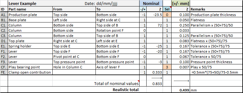
The tolerance pool in TolStackUp is a central sheet from which all tolerances are ‘fetched’ via a reference. This allows you to use the same tolerance in multiple chains without complicated administration. The screenshot below shows the result. I have hidden some superfluous columns for clarity. On the left, you see three columns with the dimensions and tolerances as they appear on the drawing. Next to them you see a code (A1., B1., etc.), the name of the part, and the interfaces. The yellow-colored columns are automatically calculated, and in the right column you can add comments. All gray columns can be filled in freely.
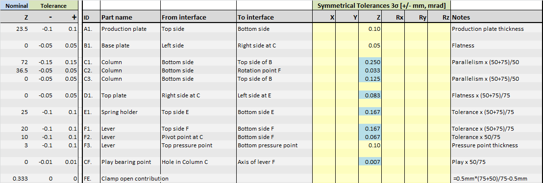
Complete tolerance table in TolStackUp.
For all contributions that are not one-to-one but are amplified by the lever, I modified the formula and colored the cell darker. Another method you could use here is the ability to define vectors in TolStackUp. These vectors are then the amplification or attenuation factors of the lever. These vector definitions are entered into the vector pool and can then be used in the 6DOF tolerance table of TolStackUp. I’ll describe this in a future article.
Complete Tolerance Chain
Each tolerance in the tolerance pool has a unique code. This makes it very easy to fill in the final tolerance chain in TolStackUp: just enter the corresponding code for each contribution in the chain (in the first column) and the whole chain will be filled in automatically.
All you have to do now is look at the two small gray columns and adjust them if necessary:
- To sum nominal dimensions, you can indicate to the left of the nominal dimension whether it should be counted in the positive (+1) or negative (-1) direction. The total gives the nominal opening of the clamping mechanism. The two dimensions of the pivot do not count. I set them to 0. The option to set the value to 0 is provided in release 2.2.0 of TolStackUp, in earlier releases you can delete the value in the corresponding cell.
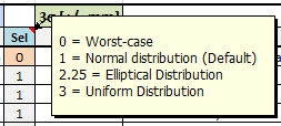
- In the ‘sel’ column, between Nominal dimension and Tolerance, you can select the summation method. The choices are statistical (normal, random, or elliptical distributed) or worst-case, see the figure below.
Which Method of Adding Tolerances
I have made the following choices:
- By default, I assume normally distributed deviations from the nominal dimension. This is most likely for controlled manufacturing processes. There may be only one or a few clamp mechanisms made for the plant. But hopefully in a controlled process and therefore a normal distribution is plausible.
- For the production plate tolerance contribution, I have chosen a worst case contribution (value 0 in the column). It is plausible that in automated production processes the deviations in plate thickness will be normally distributed. But not just one plate will be clamped, but many plates. So the probability that a plate with the maximum thickness has to be clamped is very high. And this plate must also fit into the clamp.
- I have specified the clearance in the pivot as randomly distributed (uniform, value 3 in the column). This is somewhat arbitrary, and you can completely work out how the clearance is transmitted in this clamping mechanism. I did not do that, because the contribution in the addition gives at most a few microns difference. This is something that will be discussed in a future article.
The tolerance stackup in TolStackUp is shown in the figure below.
Detailed tolerance stackup analysis table in TolStackUp.
You can immediately see the result: the nominal critical dimension K is 0.833 mm and a maximum variation of +/-0.499 mm (~3σ) can be expected.
Evaluating the Tolerance Chain
All that remains is to evaluate the result. In TolStackUp, all you have to do is enter the specification for the critical dimension and it automatically calculates the performance of the tolerance chain, the capability and an estimate of the failure rate.
The Specification
Defining the specification can sometimes be tricky, but fortunately not in this elaborate example. The production plate either fits or it doesn’t. As you can see from the summed nominal critical dimension, the clamp opening is designed to be 0.833 mm. This nominal opening can vary by +/-0.499 mm according to the analysis performed. You can now conclude that the thickest production plate, the one at the very edge of its specification, will still fit easily. The lower limit of the specification is therefore -0.833 mm. The upper limit is unimportant if a (much) too large gap is not a problem. So you can set the upper limit to any high value. I chose +10 mm.
When you fill in these two specifications, you get the complete result, see the figure below.
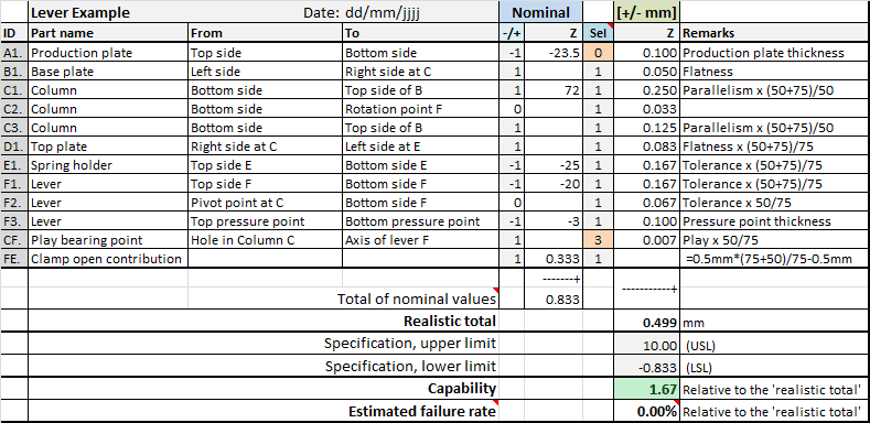
Complete tolerance table in TolStackUp with capability and failure rate.
As you would expect based on the summation of +/-0.499 mm, there is quite a margin to the specification. The expectation now is that there is a very small chance that a production plate with the largest thickness variation, the thickest possible plate, will not fit. The estimated probability of this is rounded to 0.00% (0.00000169%).
Capability and Failure Rate
Capability is a number that represents the relative performance of the chain to the specification. In formula form, it is simply: capability = specification/variation. So in this case it is 0.833/0.499 ≈ 1.67. A value greater than 1 is good and a value less than 1 is not good. The capability of 1.67 is well above 1. This leaves room for small errors and oversimplifications you may have made in your tolerance analysis. A limit of 1.3 is often used for capability. The estimated failure rate gives a more accurate picture of the impact. Capability is very useful for comparing tolerance chains and to set a consistent requirement for tolerance analysis in your company.
Practice yourself?
Want to get started with tolerance analysis? Then take this example and work it out by choosing the critical dimension for the closed state. Then calculate the distance between spring holder E and lever F. The nominal dimension is then 0.5 mm, as we saw above. And the expected variation is not 0.833 mm, but smaller. However, it should result in the same capability and failure rate.
Having trouble figuring it out? Feel free to send me an email with your question(s).